Geometry, Algebra, and Intuition

I have a confession to make: I have always found symbolic algebra more intuitive than geometric pictures. I think you’re supposed to feel the opposite way, and I greatly admire people who think and communicate in pictures, but for me, it’s usually a struggle.

For example, I have seen many pictorial “proofs without words” of the Pythagorean Theorem. I find some of them to be quite beautiful, but I also often find them difficult to unpack, and I never really think “oh, I could have come up with that myself.”

Here’s Pythagoras’ own proof^⊕Image by William B. Faulk, lifted from the Pythagorean Theorem Wikipedia Page. It’s worth looking at some of the many other visual proofs given there.:

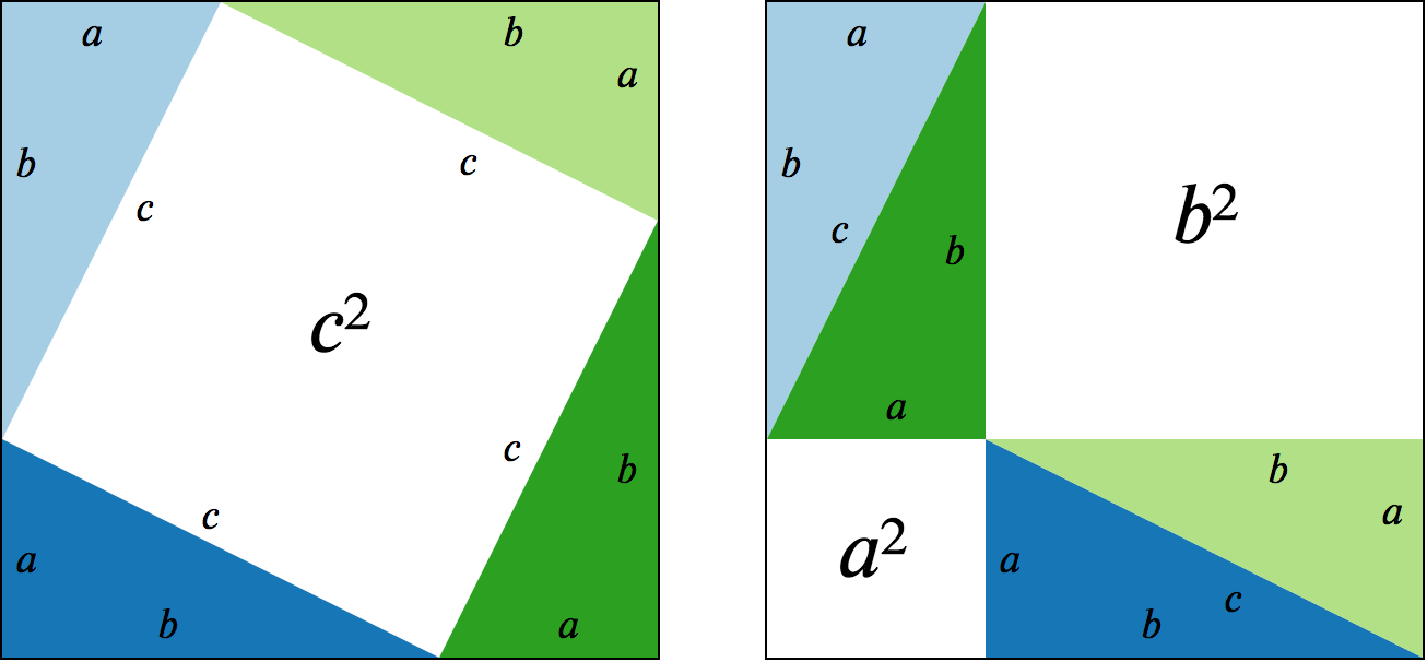
I like this proof a lot. It’s fairly simple to interpret (more so than some of the other examples in the genre), and quite convincing. We have

because, along with the same four copies of a triangle, both sides of this equation fill up an identical area.

Even so, it’s odd to me that this diagram involves four copies of the triangle. This is one of those “I couldn’t have come up with this myself” stumbling blocks.

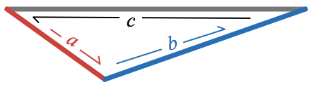
For comparison, I’ll give an algebraic proof^⊕Here and throughout I am using the word “proof” quite loosely. Forgive me, I am a physicist, not a mathematician. of the Pythagorean theorem using vectors. The condition that three vectors a, b, and c traverse a triangle is that their sum is zero:

Solving for c gives

and then dotting each side with itself and distributing gives

The condition that vectors a and b form a right angle is just that a \cdot b = 0, and in that special case, we have the Pythagorean theorem:

The thing I like about this algebraic manipulation is that it is a straightforward application of simple rules in sequence. There are dozens of ways to arrange 4 congruent triangles on a page (probably much more than dozens, really), but the algebra feels almost inevitable^⊕It does take practice to get a feel for which rules to apply to achieve a given goal, but there are really only a few rules to try: distributivity, commutativity, associativity, linearity over scalar multiplication, and that’s about it..

1. Write down the algebraic condition that vectors forming the sides of any triangle must satisfy.
2. We’re interested in a function of one of the side vectors, c^2, so we solve for c and apply the function to both sides.
3. We transform the right hand side by applying distributivity of the dot product across addition, and commutativity of the dot product, i.e. a \cdot b = b \cdot a.
4. Right triangles in particular are a simplifying special case where one term drops out.

I also think it’s important that the algebraic manipulation embeds the Pythagorean theorem as a special case of a relationship that holds for all triangles: the Law of Cosines^⊕The following diagram shows the relationship between the vector form of the law of cosines, c^2 = a^2 + b^2 + 2 a \cdot b, and the angle form of the law of cosines, 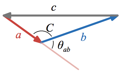c^2 = a^2 + b^2 - 2 |a||b|\cos C In the angle form, C is an interior angle, but in the vector form, if a \cdot b = |a||b|\cos(\theta_{ab}), then \theta_{ab} is an exterior angle. This is the origin of the difference in sign of the final term between the two forms.. If you have a theorem about right triangles, then you’d really like to know whether it’s ever true for non-right triangles, and how exactly it breaks down in cases where it isn’t true. Perhaps there’s a good way to deform Pythagoras’ picture to illustrate the law of cosines, but I don’t believe I’ve seen it.

For these reasons, I’ve generally been satisfied with the algebraic way of thinking about the Pythagorean theorem. So satisfied, I recently realized, that I’ve barely even tried to think about what pictures would “naturally” illustrate the algebraic manipulation.

In the remainder of this post, I plan to remedy this complacency.

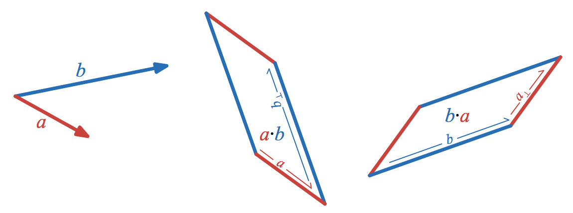
The first illustration challenge is that it’s actually kind of subtle to draw a picture that represents the magnitude of the dot product between two different vectors. E.g. given a picture showing two different vectors a and b, how exactly do you draw a picture of their dot product, a \cdot b? The dot product is related to the orthogonal projection of one vector onto the other, but it is not equal to that projection.

Orthogonal projections:

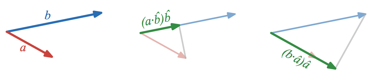
The issue is that the dot product is linear in the magnitude of both a and b, but each orthogonal projection (there are two of them) is linear in the magnitude of only one of the two vectors, and is independent of the other.

The dot product is also related to the cosine of the angle between the vectors, but again, it is not equal to either this angle or its cosine.

To make progress here, it’s useful to step back and think about exactly what pictorial proofs of the Pythagorean theorem represent.

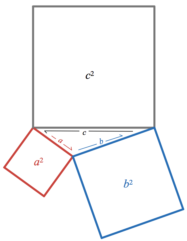
These pictures have a common feature: they represent a^2, b^2, and c^2, which we might otherwise think of as plain old numbers on the number line, by areas. And not just any areas, but squares: areas spanned by one vector, and another orthogonal vector with the same length.

Taking a leap of faith, we can try to extend this prescription for pictorially representing the square of a vector (the dot product of a vector with itself) to the dot product of a vector with a different vector. To pictorially represent the dot product, a \cdot b, form the parallelogram spanned by one of the vectors and a copy of the other vector rotated by 90 degrees.

This turns out to work, and I’m planning to give a few different reasons why in a future post. For now, you might like to try to come up with your own proof, or you might like to just take my word for it.

Applying this insight to the law of cosines gives the following pictorial formula:

Given

Then

This is fine, but the difficulty is that there are again many, many possible ways to arrange this combination of three different squares and two copies of the same parallelogram generated by the legs of our triangle, and most of them don’t make the truth of the formula visually apparent.

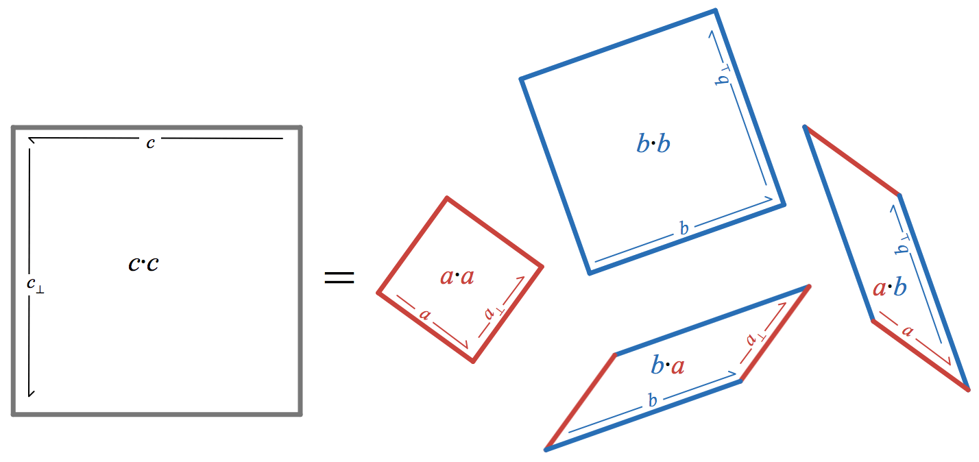
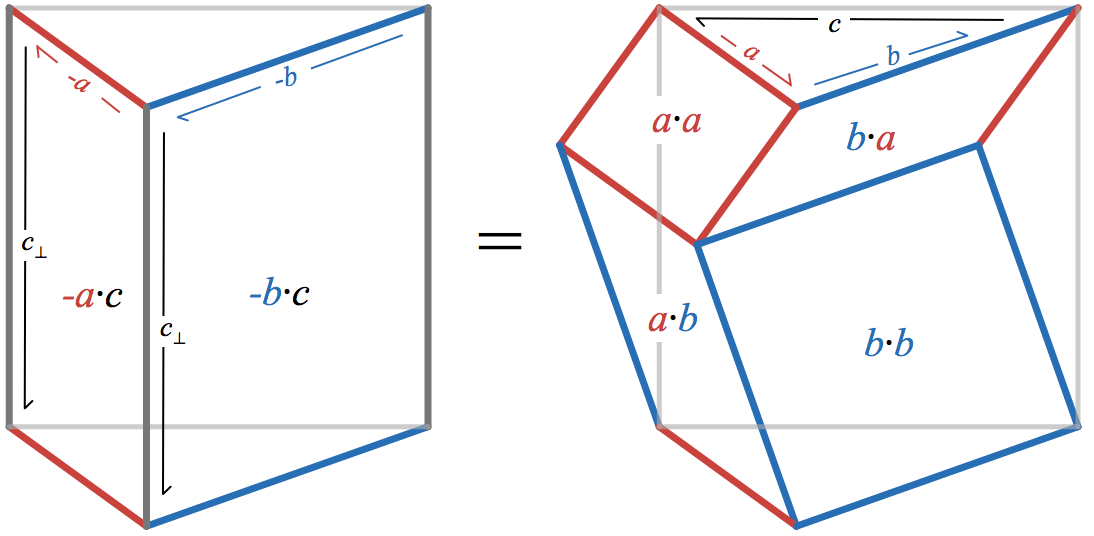
We can improve the situation by taking inspiration from the algebra to “derive” a sensible diagram through a series of steps.

Step 1

Since c = -(a + b), dotting on both sides by c gives c \cdot c = -(a + b) \cdot c and distributing gives c \cdot c = - a \cdot c - b \cdot c

You can see that this is true pictorially by dissection: if you cut a copy of the triangle out of the top of the square and paste it onto the bottom, you get a figure that’s the union of two parallelograms which must therefore have the same total area as the square; but it is also an expression of the fundamental algebraic property of distributivity^⊕Seeing this geometric property as algebraic distributivity makes it much easier to extend to cases involving products where each term might contain the sum of two or more vectors. As the situation becomes more complicated, reasoning by pictorial dissection gets out of hand faster than expanding algebraic products..

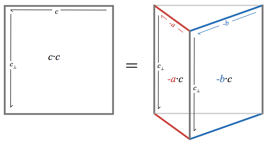
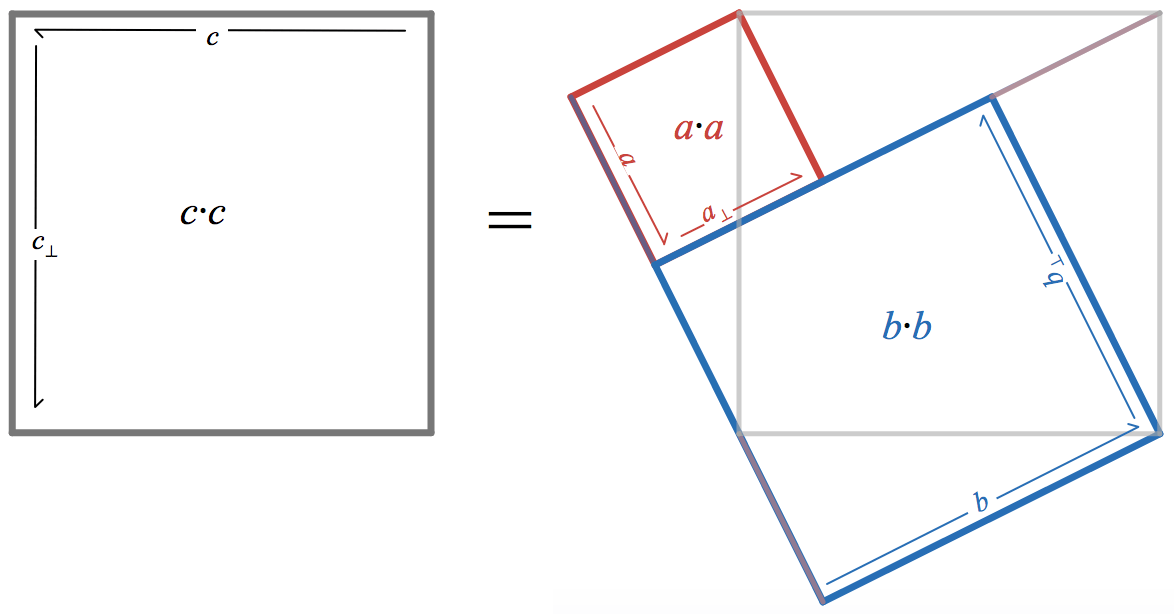
Step 2

Now use exactly the same trick to expand the c_{\perp} legs of each parallelogram into -a_{\perp} - b_{\perp} and distribute.

In algebra:

In a picture:

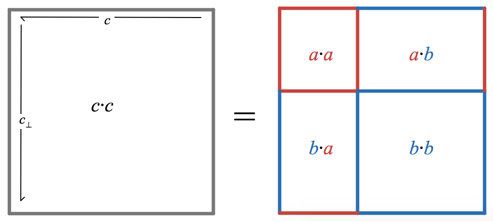
So here we finally do have a diagram that makes the law of cosines visually apparent.

The gray square is equal to the sum of the red and blue squares and parallelograms because we can form one from the other by dissection. Cut out a triangle from the top of the the gray square, and place it on the bottom. Cut out another copy of this triangle (rotated by 90 degrees) from the right side of the gray square, and place it on the left side. This procedure produces the area filled by the red and blue squares and parallelograms.

There are some nice special cases of this picture.

When a and b form a right angle, the parallelograms disappear, and we have a pictorial demonstration of the Pythagorean Theorem.

I find this one a little trickier to understand than Pythagoras’ picture in the introduction, but it works according to the same dissection argument that makes the general case work, and it has the advantage of being embedded as a special case of a diagram that depicts the law of cosines.

When a, b and c become proportional to one another (i.e. when they are all parallel or anti-parallel), we have a pictorial demonstration of the scalar identity

So far, all the triangles I have shown have either been obtuse (they have one interior angle larger than 90 degrees), or right (they have one angle equal to 90 degrees). In the case of an acute triangle (all interior angles less than 90 degrees), the diagram becomes more complicated:

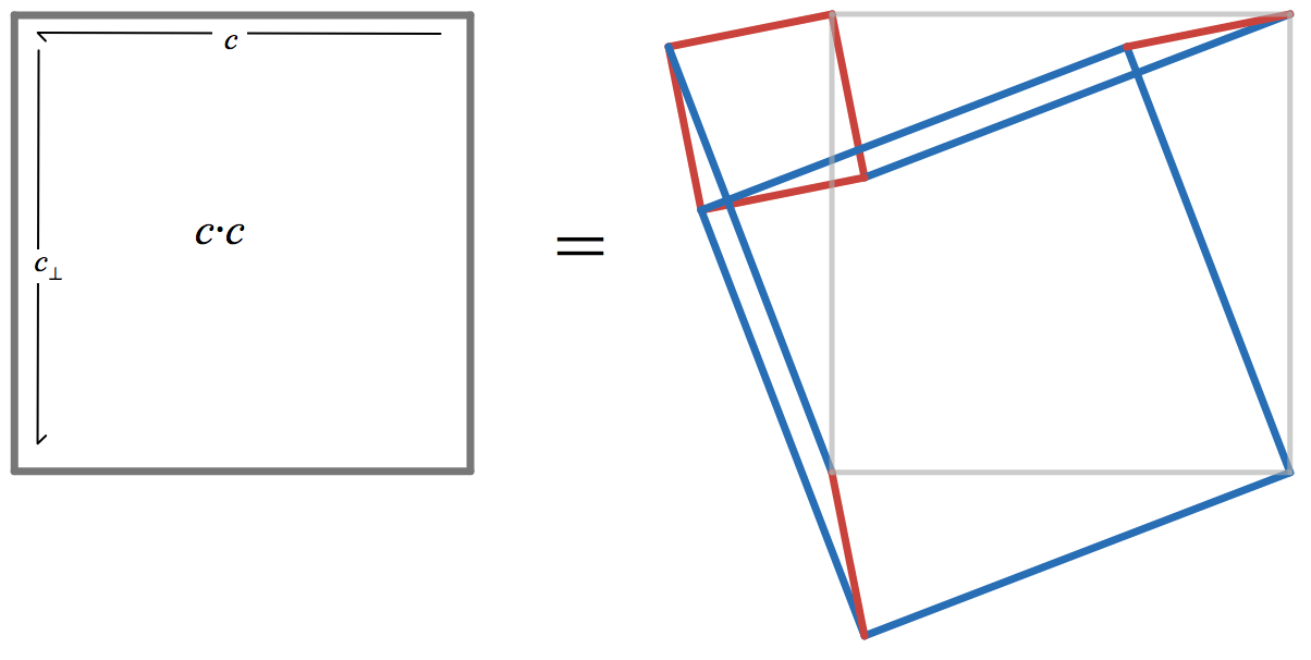
In the acute case, the dot product a \cdot b becomes negative, and so the parallelograms must be interpreted as having negative area.

This case shows the importance of taking orientation into account. If you take care to orient the sides and faces consistently, the parallelogram faces will be oriented clockwise when the square faces are oriented counterclockwise, and so their areas will have opposite signs. Failing to recognize orientation in geometry has similar consequences to failing to recognize negative numbers in arithmetic: an unnecessary proliferation of special cases in algebra and theorems.

Conclusion

I’m very happy to have discovered a picture that nicely illustrates how the Pythagorean theorem is embedded into the law of cosines, and that corresponds so closely to the algebraic way of thinking. I’d like to explore this process of “deriving pictures” further and see what I can find. I’d also like to tell you more—much, much more—about the Geometric Algebra behind the correspondence between dot products and areas of associated parallelograms, but I think I will save that for another day.

Though I still feel more comfortable “doing algebra” than “doing pictures”—I doubt this will ever really change—struggling to put the two in close correspondence has strengthened my understanding of both.

Algebra is a powerful tool for manipulating ideas, but pictures often seem to be the more powerful tool for communicating ideas. And there’s no better way to improve your own understanding of something than to attempt to communicate it.

Or as Hestenes put it, “Geometry without algebra is dumb! Algebra without geometry is blind!”

Thanks to Jacob Rus for an interesting discussion that led me to write these ideas down carefully, Bret Victor for inspiring me to work harder at making diagrams, and especially to Jaime George, who has edited this post and also all of my other posts, and who I should have thanked sooner for doing this!

Updates

Nick Jackiw points to some prior art:

Your dissection with the vanishing parallelograms is very close to Erwin Dintzl (1939). The late 19th and early 20th century, basically up to the time Hilbert’s ideas spread into curricula of the German gymnasiums, is an incredibly fertile time for geometric construction/interpretation/dissection of more modern results.

Daniel Scher writes on Twitter:

Dan Bennett has a nice activity in Pythagoras Plugged In that focuses on this visualization of the Law of Cosines.

(See the Tweet for a photograph of the relevant book page.)

Several folks contributed interactive versions of the Law of Cosines construction:

• Gray Crawford, Geogebra (via Twitter)
• Daniel Scher, Web Sketchpad (via Twitter)
• Harold Cooper, Custom JS+SVG (via Twitter)